Model-Agnostic Meta-Learning for Fast Adaptation of Deep Networks
This is a meta-learning algorithm that’s meta-agnostic i.e., it’s compatibe with any trained model and applicable to different problems including RL, regression and classification
- Year: 2017
- https://arxiv.org/pdf/1703.03400.pdf
This is a meta-learning algorithm that’s meta-agnostic i.e., it’s compatibe with any trained model and applicable to different problems including RL, regression and classification
- On a trained model, a small number of gradient steps with small training data from a new task will produce good performance generalization on that new task.
- Gives few-shot classification and regression, and accelerates fine-tuning for Policy Gradient (PG) RL
1. Introduction
- In meta-learning, the trained model’s goal is to quickly learn a new task from a small amount of new data, and the model trained on a large number of tasks
- The key idea in this work is train a model’s initial parameters such that the model has maximal performance on a new task after the parameters have been updated through one or more gradient steps computed with a small amount of data from that new task
- It doesn’t expand the parameters or constraint the architecture such as requiring RNNs. It can be combined with FCs, CNNs or RNNs
- Initializing creates an internal representation broadly suitable to many tasks such that fine-tuning the model(e.g top layer weights) can produce good results
- Authors say this work compares to SOTA one-shot supervised classification, is applicable to one-shot regression and accelerates RL in presence of task variability, substantially outperforming direct pre-training as initialization
Discussion:
Benefits of this approach:
- Simple and doesn’t introduce learned parameters for meta learning
- Can be combined with any model repsentation trainable with gradient descent and any differential objective
- Adaptation can be done with any amount of data/gradient steps
2. Model-Agnostic Meta-Learning (MAML)
2.1 Problem set-up
- A model $f$ maps an observation $x$ to an output $a$
-
This framework is applied to wide variety of different problems (classification, RL, …) so it has a generic notion of a task:
\[\mathcal{T} = \{\mathcal{L}(x_1 , a_1 , . . . , x_H , a_H ), q(x_1 ), q(x_{t+1} | x_t , a_t ), H\}\] - Each task \(\mathcal{T}\) consists of:
- A loss function $\mathcal{L}$
- A distribution over initial observations $q(x_1)$
- Transition distribuiton $q(x_{t + 1} \vert x_t, a_t)$
- Episode length: $H$
- In i.i.d. supervised learning problems, the episode length $H$ $= 1$
- It considers a distribution over tasks $p(\mathcal{T})$ that the model should adapt to.
- In the K-shot learning setting, the model is trained to learn a new task $\mathcal{T}i$ drawn from $p(\mathcal{T})$ from only $K$ samples drawn from $q_i$ and feedback $\mathcal{L}{{\mathcal{T}_i}}$ generated by $\mathcal{T}_i$
- After meta-learning, new tasks are sampled from $p(\mathcal{T})$ and meta-performance measured after learnning from K samples
2.2 MAML Algorithm
- A neural network might learn internal features broadly applicable to all tasks in $p(\mathcal{T})$, rather than to a single task (more transferable features).
- Encouraging emergence of these general-purpose representations should involve gradient-based updates making rapid progress on new tasks drawn from $p(\mathcal{T})$ without overfitting
The aim is to find model parameters sensitive to changes in the task, such that small parameters changes will produce large improvements on the loss function of any task drawn from $p(\mathcal{T})$, when altered in the direction of the gradient of that loss
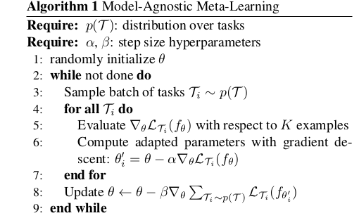
Figure 1: Model agnositic meta-learning for Few Shot Supervised Learning
-
When adapting to a new task, the parameters $\theta$ become $\theta^\prime$
\[θ^\prime_i = θ − \alpha ∇ θ L_{\mathcal{T}_i} (f_θ )\] - Step size $\alpha$ may be a fixed hyperparam or meta-learned
- The meta-optimization task (Algorithm 1, step 8) updates tasks via SGD, with a meta-step $\beta$
- MAML involves a gradient through a gradient. This requires a backward pass through $f$ to compute Hessian-vector products
3. Species of MAML
- Domains differ in the loss function and data generation/presentation
3.1 Supervised Regression and Classfication
- Few-shot learning, in supervised tasks, aims to learn a new function using a few input/output pairs using prior data from similar tasks for meta-learning e.g Classifying a dog, with a few dog pictures given a prior of seeing many types of objects
- The horizon $H = 1$, with the model accepting a single input and producing a single output
- The task $\mathcal{T}_i$ generates $K$ i.i.d observations $\textbf x$ from $q_i$. The task loss(MSE or Cross Entropy) is represented by model output for $\textbf x$ and corresponding target values $\textbf y$ for that task
- K shot regression tasks use K input/output pairs for each task
- K shot classification tasks use K input/output pairs from each task for a total of N K data points for N way classfication
-
These loss functions are be directly inserted in the MALM algorithm. This is shown in Algorithm 2.
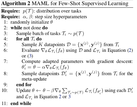
Figure 1: MAML algorithm
3.2 RL
- A new task may involve succeeding in a new environment or achieving a new goal
- The loss function corresponds to the negative expectation of the reward
- Model being learnt is a policy mapping states to a distribution over actions
4. Experiments
- For regression, the authors show MAML learns to model the periodic nature of a sine wave
- The model continues to improve with additinal grad steps, meaning it optimizes the params to lie in the region amenable to fast adaptation, and not overfitting to the params $\theta$ after one step.
Classification:
- They select $N$ unseen classes, provide the model with K different instances of each of the N classes, and evaluate the model’s ability to classify new instances.
- Tested on image classification
- Outperforms memory augmented networks and LSTM meta-learners
- The significant expense in MAML is from the use of second derivatives when backpropagating the meta-gradient
- Apparently, a first order approximation (with 2nd derivatives ommited) has almost similar performance with using full second derivatives
- This suggests most improvement comes from the post-update parameter values rather than 2nd order updates differentiating through the grad update
- Another reason is that for ReLU, 2nd derivatives may be close to zero in most cases (Authors use ReLU non-linearities)
- This removes the need for the Hessian vector product, increasing computation speed by 33%
RL (Tested in rllab):
- Net architecture: 2 hidden ReLU layers, size 100, TRPO
- 2D navigation: Agent is to move to a goal location in a 2d square
- Locomotion: Half-cheetah and Ant
- In both tasks, authors say MAML learns a model that adapts more quickly in a single gradient update and continues to improve in additional grad steps
- MAML initialization substantially outperforms random initialization and pretraining
- NOTE: Pre-training is sometimes worse than random intialization (Patisotto et al., 2016 → Deep multitask and transfer reinforcement learning).