Infer Rewards by Observing an Expert

Designing a reward function for a Reinforcement Learning(RL) task can prove notoriously difficult. No formula exists to guide reward function design – a desirable reward function is often realised through trial and error. However, that won’t always work.

Inverse Reinforcement Learning (iRL) seeks to provide an alternative to hand-engineered reward functions by recovering a suitable reward function from demonstrations of desired behaviour. This post details how iRL works and guides on the implementation of an adversarial iRL algorithm.

The need for Inverse RL

Designing a reward function in Reinforcement Learning(RL) can be troublesome. It’s simple enough that the aim is to take actions that increase the future cumulative reward and avoid those that hurt it. Choosing how to reward actions on real-world tasks, and in a way that is both learnable and expressive of the objective desired of the agent, however, is not straightforward. For example, how do you specify “acceptable” social behaviour as a function?

Inverse Reinforcement Learning (iRL) is an approach to alleviate this design problem. Instead of attempting to engineer a reward function r(s, a) ourselves, we let the RL agent observe an expert demonstrate what we wish it to learn and infer the intention of the expert from their actions. By doing so, the agent fits a reward function to the expert’s intent.

Let’s dive into this.

Our iRL implementation will connect to Generative Adversarial Networks(GANs). For this, you’ll find a basic understanding of how GANs work pretty useful, though I do brief on it below.

• The need for Inverse RL
• RL as a GAN
  • A quick detail on GANs
  • How GANs relate to inverse RL
  • Implementing training for the discriminator
  • Representing the discriminator in iRL
  • Creating a Disentangled reward function
  • Performing a Policy Update
  • iRL vs standard policy gradient algorithm
• Running inverse RL
  • Collecting expert demonstrations
  • Visualising iRL performance
• Conclusion
• References

RL as a GAN

A quick detail on GANs

A GAN comprises of a discriminator \(D\) and a generator \(G\). The generator aims to generate fake images that look as close as possible to the real images used in training. The discriminator, on the other hand, classifies a given image as either genuine or fake. So both \(D\) and \(G\) play a game where \(D\) attempts to maximize the probability that it correctly classifies an input \(x\) as real or fake, and \(G\) minimizes the likelihood that \(D\) labels its output as a fake \(1 - D(G(x))\).

The loss function that achieves this is a \(\log\) of the outputs of \(D\) and \(G\).

Where:

• \(D(x)\) – Prediction from the Discriminator if \(x\) is real/fake
• \(G(x)\) – Output from the Generator
• \(D(G(x))\) :  Prediction from the discriminator on the generator’s output

We can represent this training process as follows:

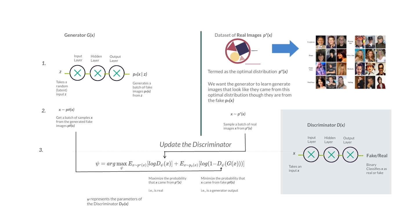
Figure 1: Stepwise representation of the working of a GAN. (Illustration by author)

How GANs relate to inverse RL

Inverse RL uses the concept of the discriminator from GANs. The discriminator in iRL is a ratio of the policy and the reward function. We see the full picture of this in a moment.

Similar to having fake images and real images in a GAN, iRL has two sets of data – the expert demonstrations and the transition data generated by the policy interacting with the environment. Both transition sets comprise state-action pairs up to a finite time step \(T\) \((s_0, a_0, s_1, a_1,\dots, s_T, a_T)\). Relating iRL to GANs, the expert demonstrations can be said to be the real data while the policy-collected samples are the fake data. Which means the policy now acts as the generator.

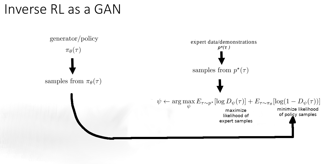
Figure 2: Inverse RL represented as a GAN. (Image modified from source)

The objective of the discriminator is represented in the same way as it is in a GAN.

Figure 3: Minmax objective of the discriminator in iRL

The first part of this objective function tries to increase the likelihood that the samples seen are expert demonstrations. The second part decreases the likelihood of the samples being collected by the running policy.

Implementing training for the discriminator

As seen, the objective in training the discriminator is to maximize the probability of correct classification of the input as real or fake. To achieve this, we maximize the loss function:

In the implementation, this is achievable in two simple steps:

1. Sample batch of expert trajectories \(τ_E\), forward pass through \(D\) and calculate the loss \(log(D(τ_E))\).
2. Sample a batch of collected policy trajectories \(τ_F\), forward-pass through \(D\) and calculate the loss \(log(D(τ_F))\). Here, we avoid doing (minimization of) \(log(1 - D(τ_F))\) because this fails to provide sufficient gradients in the learning process. So we maximize \(log(D(τ_F))\) instead.

import torch
import torch.nn as nn

BATCH_SIZE = 128


def update_discriminator(discriminator, expert_buffer, replay_buffer):
    """
        Performs a stochastic gradient update on the Discriminator
        
        Parameters
        ----------
        discriminator (nn.module): A Discriminator instance
        expert_buffer (object): A buffer holding expert demos
        replay_buffer (object): Buffer holding policy collected samples
    """
    
    # Set up loss function and optimizer
    loss_criterion = torch.nn.BCELoss()
    optimizer = torch.optim.Adam(discriminator.parameters(), lr=1e-4)

    expert_data_label = 1
    policy_data_label = 0

    # Get equal sized batches of expert and
    # policy trajectories
    expert_data = expert_buffer.sample()
    policy_data = replay_buffer.get()

    #
    # maximize log(D(x)) + log(1 - D(G(z)))

    for i in range(n_discriminator_updates):
        discriminator.zero_grad()

        # Step 1:
        # ------
        # Train D with expert data

        label = torch.full(
            size=BATCH_SIZE,
            fill_value=expert_data_label,
            dtype=torch.float32)

        # Forward pass expert data through D
        output = discriminator(expert_data)

        # Calculate loss on expert data
        # i.e., log(D(τ_E))
        loss_exp = loss_criterion(output, label)

        # Calculate gradient for D in back-pass
        loss_exp.backward()

        # Step 2:
        # -------
        # Train D with policy-collected samples

        label.fill_(policy_data_label)

        # Use D to classify policy samples
        output = discriminator(policy_data)

        # Calculate D loss on policy trajectories
        # i.e., - log(1 - D(τ_F))
        loss_pi = -loss_criterion(output, label)

        # Back-pass for gradients
        loss_pi.backward()

        total_loss = loss_pi + loss_exp

        # Update D
        optimizer.step()

Code 1: iRL discriminator update

Representing the discriminator in iRL

The discriminator \(D_{\psi}\) is a function of the reward function \(r_{\psi}\):

The discriminator in iRL: a ratio of the exponential reward function to the learned policy

\(\psi\) represents the reward function’s learnable parameters. The discriminator, being a function of the learned reward, also uses the parameters \(\psi\). Updating the discriminator D updates the learned reward function \(r(τ)\). When the discriminator is optimal, we arrive at an optimal reward function. However, the reward function above \(r(τ)\) uses an entire trajectory \(τ\) in the estimation of the reward. That gives high variance estimates compared to using a single state, action pair \(r(s, a)\), resulting in poor learning.

Using single state-action pairs will solve the high variance estimation problem but also has a drawback – it makes the optimal reward function heavily entangled with the supervised actions proposed by the optimal policy. In other words, the learned reward will encourage mimicking the expert policy and fail to produce sensible behaviour when changes occur in the environment.

That brings us to our final improvement on the discriminator.

Creating a Disentangled reward function

To extract rewards disentangled from the environment, Adversarial Inverse RL(AIRL) proposed to modify the discriminator with this form:

Discriminator using a single [state-action pair] as input

We can further simplify the reward function r(s, a, s’) to:

It’s now composed of:

1. \(g(s, a)\): a function approximator which estimates the reward of a state-action pair. It’s expressed as a function of only the state g(s) to disentangle the rewards from the environment dynamics
2. \(h(s)\): A shaping term to control undesirable shaping on g(s)

Here are the discriminator and reward function in code.

import torch.nn as nn
import torch

EPS = 1e-8


class Discriminator(nn.Module):
    """
        Classifies samples as either expert demonstrations or policy
        collected trajectores.

        It recovers the reward function r, used in updating the
        policy.

        r = g(s) + gamma * h(s') - h(s)

            where,

            g(s): Reward function approximator

            h(s): Reward shaping term

            gamma: Discount factor on value function estimate

        r is essentially an advantage A(s, a) estimate
    """

    def __init__(self, obs_dim, gamma=.99, **args):
        super(Discriminator, self).__init__()
        self.gamma = gamma

        # *g(s) = *r(s) + const
        #  g(s) recovers the optimal reward function +  some_constant
        self.g = mlp(input_size=obs_dim, output_size=1, hidden_layers=[32])

        # *h(s) = *V(s) + const (Recovers optimal value function + some_constant)
        self.h = mlp(input_size=obs_dim, output_size=1, hidden_layers=[32, 32])

        self.sigmoid = nn.Sigmoid()

    def estimate_reward(self, data):
        """
            Returns the estimated reward function / Advantage
            estimate. Given by:

            r(s, a, s') = g(s) + gamma * h(s') - h(s)


            Parameters
            ----------
            data (dict)    | [obs, obs_n, dones]
        """
        obs, obs_n, dones = data['obs'], data['obs_n'], data['terminals']
        g_s = torch.squeeze(self.g_theta(obs), axis=-1)

        # Estimate the reward
        apprx_rew = self.g(obs)
        apprx_rew = apprx_rew.squeeze()

        # Estimate the shaping term
        shaping_term = self.gamma * \
            (1 - dones) * self.h(obs_n).squeeze() - \
            self.h(obs).squeeze(-1)

        recovered_rew = apprx_rew + shaping_term

        return recovered_rew

    def forward(self, log_p, **data):
        """
            Implements the Discriminator D

                D = exp(f(s, a, s')) / [exp(f(s, a, s')) + pi(a|s)]


            Calling self(input) classifies `input` as expert_data or
            policy_samples using the Discriminator D
            Parameters:
            ----------
            log_p (torch.Tensor): Represents log[pi(a|s)]
            data (dict): Holds states, next_states and terminals
        """

        adv = self.estimate_reward(data)

        # exp(r(s, a, s'))
        exp_adv = torch.exp(adv)

        # exp(f(s, a, s')) / [exp(f(s, a, s')) + pi(a|s)]
        value = exp_adv / (exp_adv + torch.exp(log_p) + EPS)

        return self.sigmoid(value)

Code 2: Reward function implementation

\(g(s)\) recovers the optimal reward; \(h(s)\) resembles a value function. It’s therefore possible to recover the advantage from the reward function. \(r(s, a, s\prime) = \overbrace{ g(s) + \gamma h(s\prime) }^\text{Q value} - \underbrace{h(s)}_\text{Value function} = \underbrace{A(a, s)}_\text{Advantage}\)

Recovering the advantage \(A(s, a)\) from the learned reward function

Performing a Policy Update

A policy update involves finding the gradient of the log of the policy, multiplied by the advantage.

In iRL, since we aren’t observing environment rewards, which are used when estimating advantages, the change during the update will be using the reward function to approximate these advantages. More simply, the advantage recovered by the reward function finds use in the policy update.

Policy update using advantage estimation in iRL

iRL vs standard policy gradient algorithm

For an intuitive overview of iRL, here’s a side-by-side comparison of the entire pseudo-code between vanilla policy gradient(VPG), and inverse RL applied to VPG.

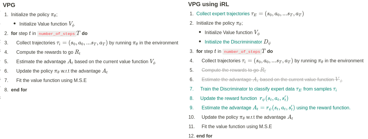
Figure 4: Vanilla Policy Gradient(VPG) compared VPG with inverse RL. iRl-added steps are in green

The policy \(π\) is trained to maximize this estimated reward \(r(s, a, s')\), and when updated, learns to collect trajectories that are more indistinguishable from the expert demonstrations.

Running inverse RL

Collecting expert demonstrations

The first step for training on inverse RL is running a policy-based RL algorithm to collect expert demonstrations. I approached this in two ways:

1. Collect the trajectories of the final n policy updates. For instance, if training for 250 epochs, collect 230–250 (last 20). That was the approach in the AIRL paper
2. Collecting trajectories whose average episode reward is above a certain reward threshold

The above two options for collecting expert data did not seem to have a notable difference in the resultant inverse RL average return (at least within 250 epoch runs). My interpretation for this being that the reward threshold in (b) collected trajectories that mostly occur in the final training episodes seen in (a).

Visualising iRL performance

Here’s a smoothed performance of iRL on HalfCheetah-v2 over 100 steps, using expert data from the five final epochs.

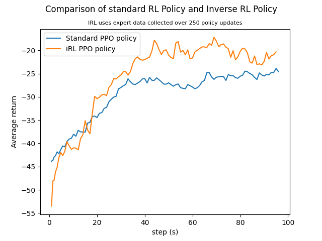
Figure 5: Half-Cheetah reward comparison of iRL policy and the same policy using observed rewards.

The complete implementation and reproduction details are on Github.

Conclusion

Inverse Reinforcement Learning allows us to demonstrate desired behaviour to an agent and attempts to enable the agent to infer our goal from the demonstrations. Aligning this goal to the demos recovers a reward function. The recovered reward, then, encourages the agent to take actions that have a similar intent to what the expert was trying to achieve.

The benefit of recovering the intent is that the agent learns the most optimal way of reaching the goal - it does not blindly copy the expert’s sub-optimal behaviour or mistakes. As a result, iRL promises more desirable performance compared to the expert policy.

References

[1] C. Finn, P. Christiano, P. Abbeel, and S. Levine. A connection between generative adversarial networks, inverse reinforcement learning, and energy-based models , NIPS, 2016.

[2] J. Fu, K. Luo, S. Levine, Learning Robust Rewards with Adversarial Inverse Reinforcement Learning , ICLR 2018.

[3] X. Peng, A. Kanazawa, S. Toyer, P. Abbeel, S. Levine, Variational Discriminator Bottleneck: Improving Imitation Learning, Inverse RL, and GANs by Constraining Information Flow , ICLR, 2019.